While Excel’s XLOOKUP function does not natively support multiple criteria directly like a built-in argument, you can combine XLOOKUP with array formulas or helper functions such as FILTER to achieve a lookup based on multiple conditions.

There are two common methods to perform a lookup with multiple criteria using XLOOKUP:

• Concatenate the Criteria into a single lookup value.
• Using a Combination of XLOOKUP and FILTER.

Method 1: Concatenate the Criteria

You can combine multiple criteria into one by concatenating them and then using XLOOKUP.

Example

Let’s say you have the following table and you want to look up the price of a product based on both Product and Category:

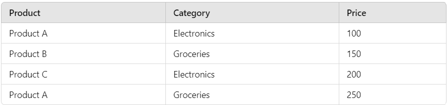
In this case, we want to look up the price of Product A in the Groceries category.

• Concatenate Criteria: You can concatenate Product and Category in the lookup value and also in the data range.
• XLOOKUP Formula: Use XLOOKUP on the concatenated values.

=XLOOKUP("Product A" & "Groceries", A2:A5 & B2:B5, C2:C5, "Not Found")

• lookup_value: "Product A" & "Groceries" combines the product and category for the lookup.
• lookup_array: A2:A5 & B2:B5 concatenates the columns of Product and Category in the lookup array.
• return_array: C2:C5 returns the corresponding Price.
• If no match is found, it returns "Not Found".

In this case, it will return 250, which is the price of Product A in the Groceries category.

Note: This method uses the concatenation (&) to combine the lookup arrays. Since this creates an array, you might need to press Ctrl + Shift + Enter for older Excel versions (prior to Excel 365 or Excel 2019).

Method 2: Using XLOOKUP with FILTER

You can use FILTER to select only the rows that match multiple criteria, and then use XLOOKUP on the result.

Example

Let’s say we have the same table, and we want to lookup the price of Product A in the Groceries category. Here’s how you would use FILTER to create a filtered list and use XLOOKUP to get the price.

=XLOOKUP(TRUE, (A2:A5="Product A") * (B2:B5="Groceries"), C2:C5, "Not Found")

• lookup_value: We are looking for TRUE since XLOOKUP expects to match a single condition.
• (A2:A5="Product A") * (B2:B5="Groceries"): This creates a Boolean array where both conditions must be TRUE. The multiplication (*) acts as an “AND” operation to ensure both conditions are met.
• return_array: C2:C5 returns the Price where both conditions match.

In this case, it will return 250, which is the price of Product A in the Groceries category.

Bonus: Using FILTER with XLOOKUP

Alternatively, you can use the FILTER function to return all rows that meet multiple conditions and combine it with XLOOKUP:

=FILTER(C2:C5, (A2:A5="Product A") * (B2:B5="Groceries"), "Not Found")

This will return 250 for Product A in Groceries.

• Method 1 (Concatenation): Concatenates the multiple criteria into a single value and uses XLOOKUP on the concatenated arrays.

• Method 2 (XLOOKUP with FILTER): Creates a Boolean condition based on multiple criteria and searches where both criteria are true.