How to use ACOSH function in excel

Posted on: April 18, 2021 in Excel , Excel Functions ,

Description

The ACOSH function is a built-in function in MS Excel (Microsoft Excel), which is classified as a math / trig function.

The ACOSH function returns the inverse hyperbolic cosine of a number.

This is one of the worksheet function. It can be used as a worksheet function in Excel.

Return value

This function returns the inverse hyperbolic cosine of a number.

Syntax


=ACOSH(number)

The number must be greater than or equal to 1. The inverse hyperbolic cosine is the value whose hyperbolic cosine is number, so ACOSH(COSH(number)) equals number.

Note: The number must be greater than or equal to 1. Otherwise #NUM! returns an error.
If number is not numeric, then #VALUE! is returned.

See an example picture of this function

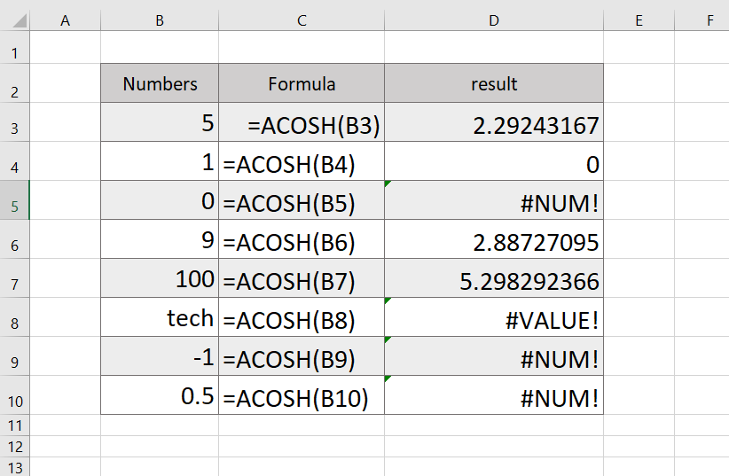
Table content

Formula	Description	Result
=ACOSH(10)	Inverse hyperbolic cosine of 10	2.99322284612638
=ACOSH(C5)	Inverse hyperbolic cosine of C5 cell value	0
=ACOSH(“tech”)	Number is not numeric, Return #VALUE! Error	#VALUE!
=ACOSH(-1)	Return #NUM! Error	#NUM!
=ACOSH(0.5)	Number < 1 Return #NUM! Error	#NUM!