How to use AVERAGE Function in Excel.

Description
This function calculates the average from a list of numbers.
Arguments can either be numbers or names, ranges, or cell references that contain numbers.
Logical values and text representations of numbers that you type directly into the list of arguments are counted.
AVERAGE function can handle up to 255 individual arguments, which can include numbers, cell references, ranges, arrays, and constants.
If an [group of selection]array or cell reference argument contains text, logical values, or empty cells, those values are ignored. However, The value of that cell is zero are included.
Arguments that are error values or text that cannot be translated into numbers cause errors.
If you want to include logical values and text representations of numbers in a reference as part of the calculation, use the AVERAGEA function.
If you want to calculate the average of only the values that meet certain criteria, use the AVERAGEIF function or the AVERAGEIFS function.
Return value
Returns the average of the arguments.
Syntax
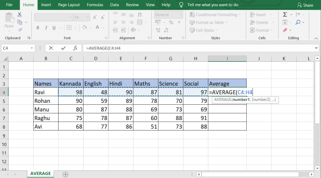
=AVERAGE(number1, [number2], ...)
Arguments
number1 :  A number or cell reference that numeric value.

number2 :  [optional] (this is optional) A value or reference to a value that can be evaluate as a number
For example =AVERAGE (2,5,6,7,10) returns 6.
Manual calculation method:
2 + 5 + 6 + 7 + 10 = 30 / 5 = average of numbers 6
Note: The AVERAGE function measures central tendency, which is the location of the center of a group of numbers in a statistical distribution. The three most common measures of central tendency are below :
Example
Average, which is the arithmetic mean, and is calculated by adding a group of numbers and then dividing by the count of those numbers.
For example, the average of 1, 2, 3, 4, 5, and 15 is 30 divided by 6, which is 5.
 1  +  2  +  3  +  4  +  5  +  15  =  30 (result )  average of numbers  5

30 /  6   (count of numbers) =  5  (this result is average value of numbers)
Median, which is the middle number of a group of numbers
For example, the median of 2, 3, 3, 5, 7, and 10 is 4.
Mode, which is the most frequently occurring number in a group of numbers.
For example, the mode of 2, 3, 3, 5, 7, and 10 is 3.
| Formula | Description | Result |
|---|---|---|
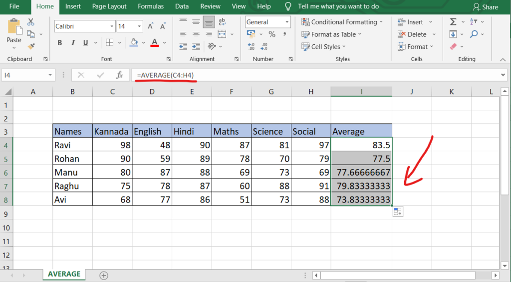
| =AVERAGE(C4:H4) | Average of the numbers in cells C4 to H4. | 83.5 |
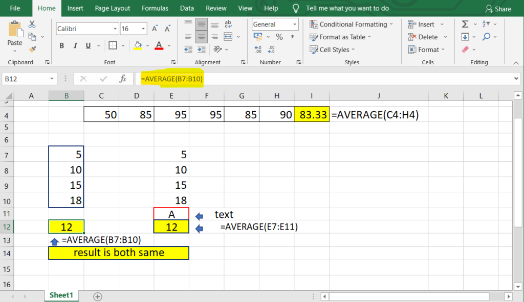
| =AVERAGE(B7:B10) | Average of the numbers in cells B7 to B10. | 12 |
| =AVERAGE(E7:E11) | Average of the numbers in cells E7 to E11. A added in E11 cell but ignored. | 12 |
Related post
-
 How to Use XLOOKUP with Multiple Criteria in Excel
While Excel’s XLOOKUP function does not natively support multiple criteria…
-
 How to Use XLOOKUP in Excel
XLOOKUP is a versatile function in Excel used for performing…
-
 How to use LOWER Function in Excel
Excel Lower Function Converts all uppercase letters in a text…
-
 How to use ADDRESS Function in Excel
The ADDRESS function to obtain the address of a cell…
-
 How to use ACOSH function in excel
The ACOSH function returns the inverse hyperbolic cosine of a…
Popular post
-
 Eclipse IDE – Create New Java Project.
Opening the New Java Project…
-
 How to start the project in android studio
Android Studio Open the Android…
-
How to use ACOSH function in excel
The ACOSH function returns the…
-
 Complete Header tags in html – easy to learn
H tags can be used…
-
 Best features in Python programme – easy to learn
Python is the most widely…